Geometry#

Polygon mesh and Half-edge data structure#

Triangle mesh: Vertex table + Edge table + Triangle table

Half-edge structure:

struct HalfEdge {
  HalfEdge *twin; // 共边面片对应的半边
  HalfEdge *next; // 同一个面片的下一条边
  Vertex *vertex; // 边的起点或者终点，自行钦定
  Edge *edge; // 相关的边
  Face *face; // 相关的面片
}

cpp

Quad mesh:

易于差值和参数化

Subdivision surface#

Catmull-Clark#

计算新的面点和边点
$\begin{aligned} f_p & = \frac{1}{n}\sum_{v \in F} v \\ e_p & = \frac{f_1+f_2+v_1+v_2}{4} \end{aligned}$
更新顶点
$\begin{aligned} R &=\frac{1}{edge(v)}\sum_{e \owns v} \text{midpoint} (e) \\ F &= \frac{1}{face(v)}\sum_{f \owns v} f_p(f)\\ v_{new} & = \frac{F+2R+(n-3)v}{n} \quad (n=face(v)) \end{aligned}$
形成新的 Quad mesh。

面点与原始面的边点相连，新的顶点与原始点的边的边点相连。

这里可以保证细分之后的 Polygon mesh 一定是 Quad mesh。

Loop#

计算边点，如果不是边界，那么
$e_p = \frac{3}{8}(v_0+v_2)+\frac{1}{8}(v_1+v_3)$
否则就直接用中点
$e_p = \frac{1}{2}(v_0 + v_1)$
更新顶点。 $v_i$ 为 $v$ 的邻居， $n$ 是邻居数量，当 $n=3$ 时 $u=\frac{3}{16}$ 其他时为 $\frac{3}{8n}$ 。
$v' = (1 - n * u) v + u\sum_{i=1}^{n} v_i$
形成新的 Triangle mesh。

一个面的三个边点相连，原始边的边点与两个更新后的顶点相连。

Mesh Parameterization#

平均系数 $\lambda_{ij} = \frac{1}{n_i}$
均值坐标系数 $\lambda_{ij} = \frac{\tan \frac{\beta_{ji}}{2} + \tan \frac{\alpha_{ij}}{2}}{r_{ij}}$
调和坐标系数 $\lambda_{ij} = \frac{\cot \gamma_{ij} + \cot \gamma_{ji}}{2}$ ，近似于保角映射

Discrete differential geometry#

局部平均区域#

重心单元 (barycentric cell)，即把三角形的两边的中点和三角形的重心顺次连起来．
泰森多边形单元 (Voronoi cell)，是由每条边的中垂线确定的区域，根据中垂线的性质，每个三角形内，蓝色区域中的点到 x 的距离都会小于另两个顶点，若顶点周围存在钝角三角形，则蓝色区域会超出三角形．
混合泰森多边形单元 (mixed Voronoi cell) 是对上一种方法的改进，在出现钝角三角形时，用三条边的中点连线来框选出该三角形内的蓝色区域．

Normal Vector#

单个三角形的法向量是朴素的，关键是如何定义顶点的法向量。

\mathbf n(x) = \text{normalize}(\sum_{T \in \Omega(x)} \alpha_{T}\mathbf n(T))

$\alpha_T = 1$
$\alpha_T = \text{area}(T)$
$\alpha_T = \theta(T)$

三角坐标及对应的梯度#

拉普拉斯算子#

均匀拉普拉斯

(\Delta f) _i = \frac{1}{N}\sum_{j \in \Omega(i)} (f_j-f_i)

余切拉普拉斯

(\Delta f) _i = \frac{1}{2A_i} \sum_{j \in \Omega(i)}(\cot \alpha_{ij} + \cot \beta _{ij})(f_j-f_i)

梯度与拉普拉斯#

梯度：标量场 f 的变化方向

拉普拉斯：场 f 的细节

Mesh smoothing#

Diffusion equation

\frac{\partial f(\mathbf x ,t)}{\partial t} = \lambda \Delta f(\mathbf x,t)

由于 $\Delta f(\mathbf x, t)$ 在这里有离散形式，所以还可以写成矩阵的形式。

\frac{\partial \mathbf f(t)}{\partial t} = \lambda L \mathbf f(t)

对时间和空间离散，并使用显式欧拉，那么有

\mathbf x_i \leftarrow \mathbf x_i + h\cdot \lambda \cdot \Delta \mathbf x_i

余切算子能更好地保持几何特征，而均匀算子导致了三角网格切向的松弛

Mesh editing#

限制 $v'_i = u_i , i \in C$

求

\tilde{V'} = \argmin_{V'} \Big ( \parallel L(V') - L(V) \parallel^2 + \sum _{i \in C} \parallel v'_i - u_i \parallel ^2\Big)

Mesh simplification#

How much does it cost to collapse an edge?

Basic idea: compute edge midpoint, measure quadric error

Better idea: choose a point that minimizes quadric error

Quadric error: new vertex should minimize its sum of square distance (L2 distance) to previously related triangle planes!

Square distance to a single plane: $h_d^2= \tilde{v}^T \big(\frac{\mathbf{\tilde n}\mathbf{\tilde n}^T}{\mathbf n \mathbf n^T} \big) \tilde{v}$

Quadric error: sum of square distances: $\text{Error}(v) = \tilde{v}^T\sum K_p \tilde{v} = \tilde{v}^T Q \tilde{v}$

Reconstruction#

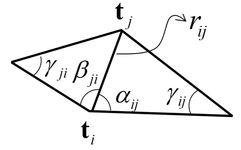
Registration#

Definition: transform one model to another based on their partially overlapping features

Alignment: find a correct transformation

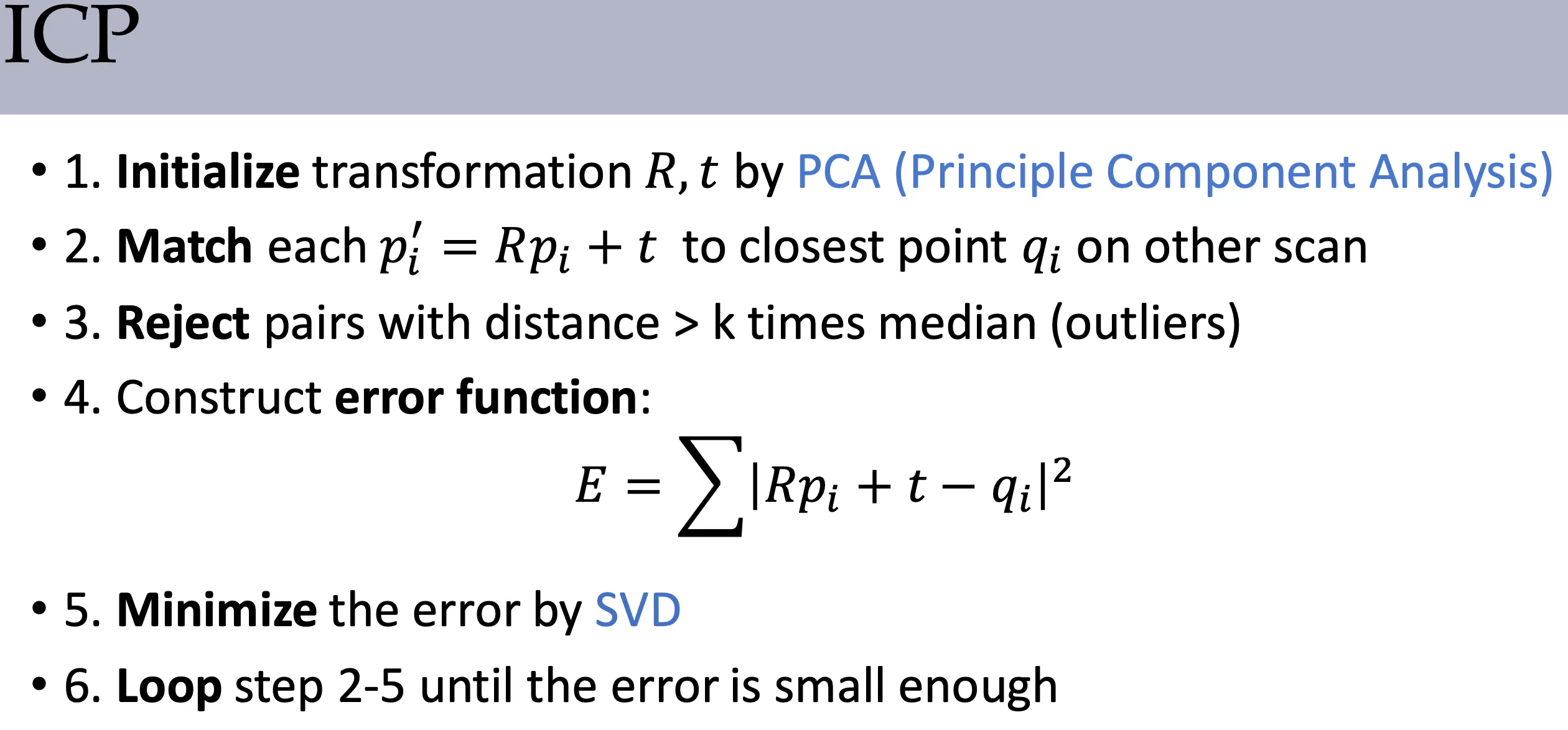
PCA:

The eigenvectors form orthogonal axes (2 vectors in 2D; 3 vectors in 3D)
Compute $R, t$ from one to another

P = \begin{bmatrix} p_{1x} - c_x & \cdots & p_{nx}-c_x \\ p_{1y} - c_y & \cdots & p_{ny} -c_y \\ p_{1z} - c_z & \cdots & p_{nz} - c_z \end{bmatrix} \\ M = PP^T

Eigenvectors of $M$ represent principal directions of shape variation.

SVD $P$ to get eigenvectors of $M$ .

Surface Reconstruction Algorithm#

Directly: Triangulation

Delaunay Triangulation

Indirectly: Implicit Surfaces + Marching Cubes

Poisson Surface Reconstruction

Delaunay:

最大化所有三角形中最小的角

最后的结果是任何三角形的外接圆内，都不包含任何点。

增量式进行，每次向当前集合中添加一个点并连接一些边组成三角形，随后检查受到影响的周围的三角形是否满足德劳内性质，并对不满足性质的三角形进行翻转。

可以通过分治算法优化。

Poisson Surface Reconstruction: 计算 SDF 然后行进立方体

假设 $\chi_M$ 是形状 $M$ 对应的 SDF，我们通过计算 $\nabla \chi_M = 0$ 来表示 $\partial M$ 。

The input is oriented points $\vec{V}$ (points with normals) sampled from a shape $M$ .

由于 $\nabla \chi = \vec{V}$ 所以 $\Delta \chi = \nabla \cdot \vec{V}$

然后估计最小二乘解。（上面的 $\Delta \chi$ 可以用矩阵形式描述）

算法通过八叉树 (Octree) 组织这些带法向量信息的点并在八叉树节点上定义一系列基函数，通过求解上述泊松方程得到基函数之间组合的系数，从而最终拟合出指示函数．

Marching Cubes:

分割若干个立方体，用 SDF 的到 256 中情况，根据不同的情况重建表面。

关于边上的点，要按照 SDF 的值来插值计算。

RANSAC#

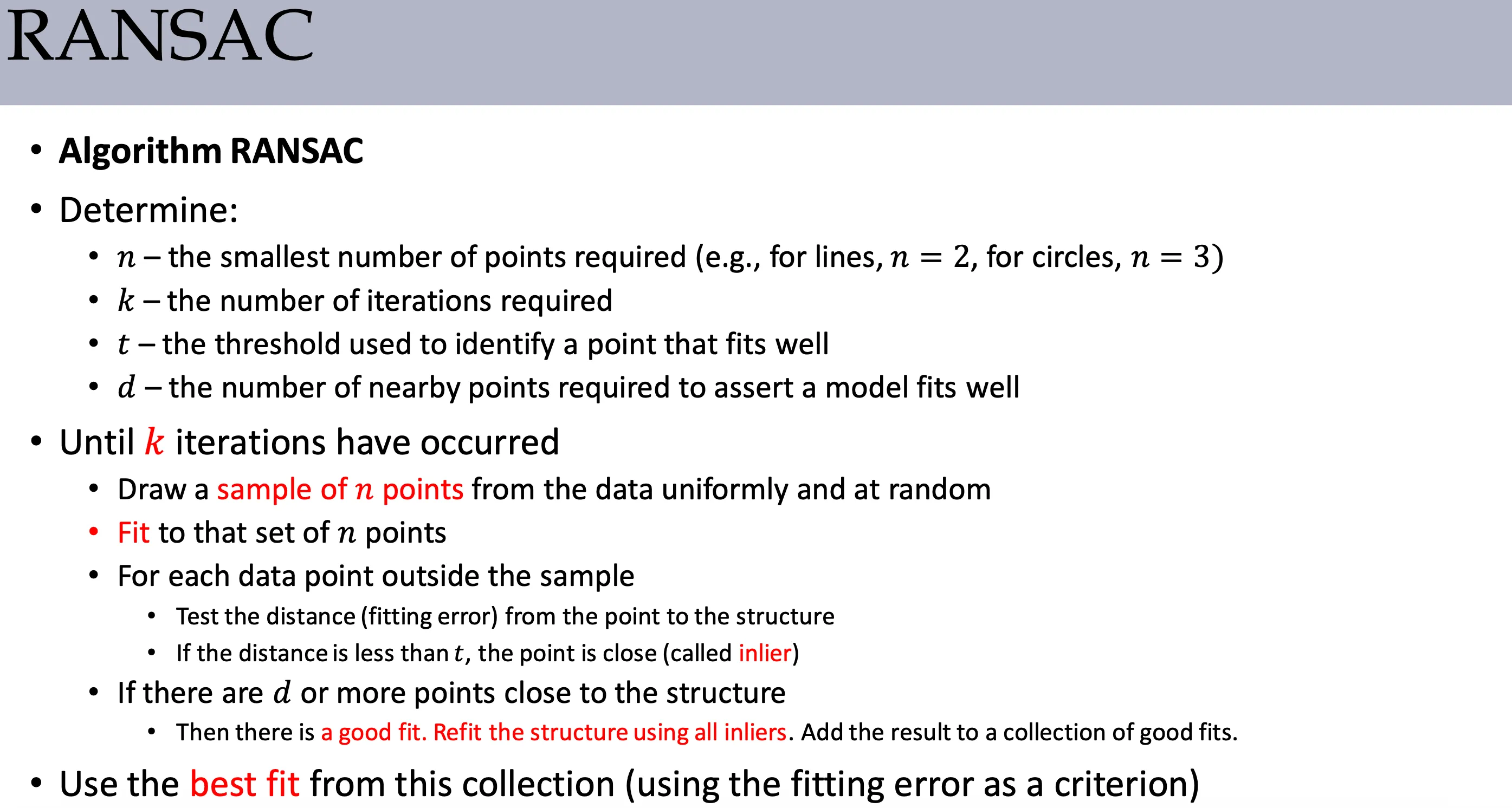
按照内点数量判断是否继续，最后用内点重新计算答案。

随机选择一个用于估算的最小子集（对于估计平面来说，该子集包含 3 个点）
用这个子集估算待求的参数
用估算的参数测试整个数据集，将误差在一定范围内的数据点作为“内点”(inliers)
如果内点的数量超过一定比例，就以全部内点为输入，使用最小二乘法重新估计一组更精确的待求参数
重复 1-4 步若干次，最后将“用最多内点估计出的参数”作为最终结果．

Transformation#

Axis-angle rotation in matrix representation#

\mathbf x' = \cos \theta \mathbf x + (1 - \cos \theta) (\mathbf x \cdot \mathbf a)\mathbf a + \sin \theta (\mathbf a \times \mathbf x)

The matrix $R$ for rotation by $\theta$ about axis (unit) $\mathbf a$ :

R = \mathbf a \mathbf a ^T + \cos \theta (I - \mathbf a \mathbf a ^T) + \sin \theta \mathbf a ^* \\ \mathbf a ^* = \begin{bmatrix} 0 & -\mathbf a_z & \mathbf a_y \\ \mathbf a_z & 0 & \mathbf -a_x\\ - \mathbf a_y & \mathbf a_x & 0 \end{bmatrix}

欧拉角#

各种变换#

Translation
Rotation
Shear
Scale
Coordinate transformation
…

用齐次坐标，全部可以写成矩阵的形式，方便复合。

二维的旋转可以分解为两个类似于剪切的变换的复合。

铰接模型 Articulated Model#

某些部位自由度受限。

有依赖关系，前面改变了后面也要改变。

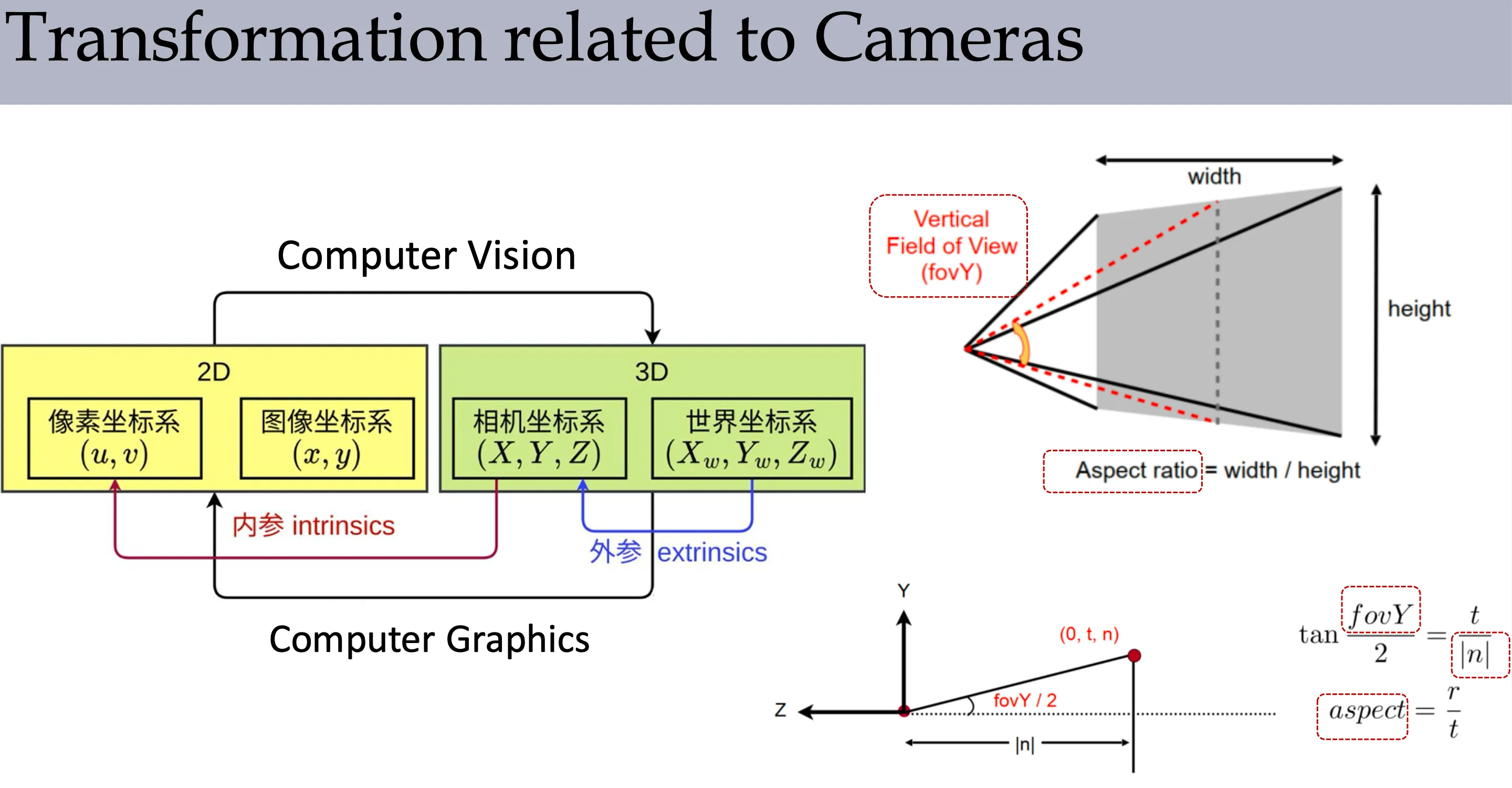
Viewing Projection#

near plane 就是成像平面

far plane 是考虑的最远的平面（渲染范围）

分为正交投影（Orthographic projection）和透视投影（Perspective projection），由于透视投影不是线性的，所以要使用齐次坐标来计算。

这里的坐标都是列向量，所以是 $P' = M P$ 。

在求透视投影的矩阵时，如何计算 $z'$ 是不知道的，但是我们知道 $z'= az+b$ ，然后用 $z_{near},z_{far}$ 来求解 $a,b$ 即可。

注意，在计算了透视投影后，在接一个正交投影映射到长方体中，然后根据 z-buffer 确定如何显示。

在真实的相机中：

Randering#

Shadow Map#

从光源视角，渲染出一张纹理图，记录最近距离。

对于要计算的一个像素（对应点 $P$ ），计算 $P$ 在光源视角的位置，并计算距离。并于纹理图比较，判断是否在阴影中。

Mipmap#

反走样的方法。

由于远处一个像素可能在纹理坐标上代表一个很大的范围，所以提前把原始的纹理图按照不同的比例压缩（多个像素的信息合并到一个像素上）。

这样根据表示范围的大小，在对应的压缩后的纹理图上提取信息，在相邻的两层之间插值。

由于可能不同方向的压缩比例不同（各向异性），所以不仅是同比例的压缩，还有不同比例压缩的组合。

法向贴图（Normal Mapping） or 凹凸贴图（BumpMapping）#

凹凸不平的表面并不影响碰撞等宏观性质，那么可以把凹凸不平的效果记录在纹理中，比如记录法向。

这样不改变表面的几何性质，但是又能正确的渲染颜色。

环境光贴图（Environment Mapping）#

考虑把周围的环境（远处的信息），用贴图表示，而不是一个几何物体，一种方法是 skybox，这样就可以快速计算环境的光照了。

注意这里要让环境的深度始终为 $1.0$ 这样才是背景，在 skybox 中强行钦定 $z=w$ 。

Ray Tracing#

一个像素只有一条 ray 会导致走样，使用 supersampling 的方法反走样。

Shadow Rays#

从要计算颜色的点 $P$ 向光源方向发射一条射线，如果撞到物体说明被遮挡。

不用计算最近交点，只要撞到任意一个不透明物体就是遮挡的。返回布尔值或者透明度。

基础光追 Whitted-style 中光源是一个点，非黑即白（硬阴影）。

现代路径追踪 Path Tracing 或者分布式光线追踪中，光源有面积，在光源表面随机采样所个点，每个点都计算 Shadow ray，然后按照比例计算亮度。

Path Tracing#

Distribution ray tracing 的一种

a ray tracing method based on integral transport equation and rendering equation

Bidirectional Reflectance Distribution Function#

f_r(\omega_i \rightarrow \omega_r) = \frac{\mathrm{d} L_r(\omega_r)}{\mathrm{d}E_i(\omega_i)} = \frac{\mathrm d L_r(\omega_r)}{L_i(\omega_i)\cos \theta_i \mathrm d \omega_i}

考虑自发光

L_o(p, \omega_o) = L_e(p, \omega_o) + \int_{H^2} L_i(p, \omega_i)f_r(p,\omega_i,\omega_o)(\mathbf{n}\cdot\omega_i) \mathrm{d}\omega_i

Monte Carlo solver: 随机若干个 $\omega_i$ 计算积分。碰到物体就递归（光追）

VCI 复习